A Simple QPM Model for Vietnam
This note summarizes the canonical Quarterly Projection Model (QPM), a small open-economy New Keynesian model used by inflation-targeting central banks for monetary policy analysis and forecasting.
Replication code HERE. If you spot any errors, please let me know.
What is the QPM?
The QPM is a semi-structural, general equilibrium, stochastic model with rational expectations. Prices are sticky, output is demand-determined in the short run, and the central bank uses the interest rate as its policy instrument.
Four Building Blocks
1. Aggregate Demand (IS Curve)
\[\hat{y}_t = b_0 E_t(\hat{y}_{t+1}) + b_1 \hat{y}_{t-1} - b_2\, mci_t + b_3 \hat{y}^* + \varepsilon_t^y\]Output gap depends on its expectations, its own lag (persistence), the monetary conditions index (MCI), and the foreign output gap. MCI is a weighted average of the real interest rate gap and real exchange rate gap:
\[mci_t = b_4\,\hat{r}_t + (1-b_4)(-\hat{z}_t)\]where \(r_t = i_t - E_t(\pi_{t+1})\)
\[z_t = s_t + p_t^\ast - p_t\]This indicates that the equilibrium values of the real interest rate and of the real exchange rate are consistent with the neutral monetary conditions. In other words, when both the real interest rate and the real exchange rate are at equilibrium levels, both gaps are 0. And then the monetary conditions index is also 0.
The real interest rate impacts decisions to substitute between consumption today and savings today to consume in the future and to borrow funds to finance investment and consumption expenditure. The real exchange rate impacts substitution or shifts in demand between domestically and foreign-produced goods, as it captures changes in relative prices.
2. Inflation (Phillips Curve)
\[\pi_t = a_1\pi_{t-1} + (1-a_1)E_t\pi_{t+1} + a_2\,rmc_t + \varepsilon_t^\pi\]Inflation is driven by backward-looking firms (weight $a_1$), forward-looking firms ($1-a_1$), and real marginal costs:
\[rmc_t = a_3\,\hat{y}_t + (1-a_3)(-\hat{z}_t)\]To produce extra unit of goods or services, at some point firms may, in particular, need to ask existing employees to work extra hours or will have to hire more employees. In this situation, the already existing workers may need to be paid more than the usual rate per unit of production. Also, higher demand for extra labor may put upward pressure on wages. Because of such wage pressures, the cost per additionally produced unit of goods and services will increase. Then firms will need to increase prices to accommodate costs and preserve profit margins and therefore domestic cost pressures on inflation will increase.
Another reason why the output gap can approximate domestic costs is because when the output gap and capacity utilization increase, then firms use their productive capacity or productive capital more intensively. Therefore, productive capital is going to depreciate quicker. And firms will need to replace capital earlier. To be able to do that, firms will have to allow for higher rates of depreciation and set aside additional financial resources. This extra costs of replacing faster depreciating capital will lead to higher marginal costs of production and higher inflation.
The real exchange rate gap approximates a real marginal cost that vary with the relative prices of imports. For example, assume that the nominal exchange rate depreciates and that the real exchange rate gap becomes more positive or less negative. The cost of imported goods in the domestic currency equivalent increases. Again, costs will be passing through to prices which will increase inflation.
3. Exchange Rate (Modified UIP)
In equilibrium, an optimizing household must be indifferent between investing in domestic or foreign assets, a condition that is captured by the following equation. \(i_t = i^\ast_t + E_t(s_{t+1}) - s_t\) What this equation is showing us is that the rate of return of 1 dollar invested in a domestic bond for one period, here represented by i at time t, must be equal to the expected rate of return of 1 converted to the foreign currency in period t at exchange rate St, which is here, then invested for one period at rate $i^\ast_t$ and reconverted to domestic currency in period $t+1$ at the expected exchange rate St plus 1.
Another way of expressing is no-arbitrage condition is seen here. \(s_t = E_t(s_{t+1}) + (i^\ast_t - i_t)\)
This simply says that the exchange rate at time t is equal to the expected level of the exchange rate in the next period and the differential between foreign and domestic interest rates.
As it turns out, the UIP in this simple form does not hold empirically, perhaps because domestic and foreign bonds are not always close substitutes, reflecting differences in liquidity and credit risk. So sometimes you have the left-hand side higher than the right-hand side of this equation. So to account for that, a wedge must be included to ensure that the two sides of the equation are equal.
If the rate of return on domestic bonds is higher than that of foreign bonds, adjusted by the expected change of the exchange rate, one can interpret the difference, or wedge, as representing the country’s risk premium.
That is, even if the return on domestic bonds is higher than that of foreign bonds, investors still will not buy domestic bonds unless they are compensated for the risk they incur, which is measured by the premium. Taking into account the fact that domestic and foreign bonds may not be perfect substitutable and the existence of a risk premium or discount, the UIP must be modified.
So the UIP condition must be modified in order to account for the risk premium from this equation to this equation. \(s_t = E_t(s_{t+1}) + i^\ast_t - i_t + prem_t\)
But since we are working with a quarterly model, and interest rates and premium are typically expressed at annualized rates, to convert them to quarterly frequency, they must be divided by 4. So the model counterpart of the UIP condition needs to be changed to this equation. \(s_t = E_t(s_{t+1}) + (i^\ast_t - i_t + prem_t)/4 + \varepsilon^s_t\)
The exchange rate can be very volatile and jumpy, especially at high frequencies, indicating that new information is readily incorporated into its determination. However at quarterly frequency, the exchange rate tends to display some inertia, consistent with some backward looking behavior. Thus, we are going to use the following specification
\[s_t = (1-e_1)E_t(s_{t+1}) + e_1[ s_{t-1} + 2(\pi^T_t - \bar{\pi}^\ast_t + \Delta \bar{z}_t)/4 ] + (i^\ast - i_t + prem_t)/4 + \varepsilon_t^s\]The UIP condition links the nominal exchange rate to the interest rate differential and country risk premium. A backward-looking component ($e_1$) captures empirical exchange rate inertia.
4. Monetary Policy Rule
\[i_t = g_1 i_{t-1} + (1-g_1)\bigl[i_t^n + g_2(E_t\pi^4_{t+N} - \pi^T_{t+N}) + g_3\hat{y}_t\bigr] + \varepsilon_t^i\]The central bank smooths the interest rate ($g_1$), reacts to expected inflation deviations from target ($g_2 > 1$, Taylor principle), and to the output gap ($g_3$). The neutral rate is $i_t^n = \bar{r}t + E_t\pi^4{t+N}$.
Estimation
- Observed: GDP, CPI, interest rates, exchange rate, inflation target
- Unobserved (estimated via Kalman filter): output gap, potential growth, equilibrium real interest rate, real exchange rate trend
Trends must satisfy two equilibrium conditions:
- PPP: $\Delta\bar{s} = \bar{\pi} - \bar{\pi}^* - \Delta\bar{z}$ — the inflation target and nominal depreciation path must be mutually consistent.
- UIP (real): $\Delta\bar{z} = \bar{r} - \bar{r}^* - prem$ — real exchange rate trend must be consistent with the real interest rate differential.
Results
| Parameter | Typical range | Posterior mode | Interpretation |
|---|---|---|---|
| $b_0$ | 0.1–0.9 | 0.083 | Output gap lead |
| $b_1$ | 0.1–0.9 | 0.593 | Output gap persistence |
| $b_2$ | 0.1–0.5 | 0.205 | Policy (MCI) pass-through to demand |
| $b_3$ | 0.1–0.5 | 0.342 | External demand pass-through to demand |
| $b_4$ | 0.3–0.8 | 0.300 | Weight of interest in MCI |
| $a_1$ | 0.4–0.9 | 0.419 | Inflation inertia |
| $a_2$ | 0.1–0.5 | 0.109 | Cost pass-through to prices |
| $a_3$ | 0.6–0.9 | 0.696 | Weight of domestic costs in RMC |
| $g_1$ | 0.0–0.8 | 0.800 | Interest rate smoothing (“wait-and-see” policy) |
| $g_2$ | 0.1–Inf | 0.427 | Weight of inflation in policy decision |
| $g_3$ | 0.1–Inf | 0.392 | Weight of output gap in policy decision |
| $e_1$ | 0.4–0.9 | 0.925 | FX backward-looking |
Interpretation of Estimation Results
Aggregate Demand (IS Curve)
The estimated output gap persistence ($b_1 = 0.593$) is moderate, indicating that business cycles in Vietnam are not excessively prolonged but do carry meaningful inertia. The forward-looking component ($b_0 = 0.083$) is small and only marginally significant ($p = 0.100$), suggesting agents form some expectations about future output conditions, though backward-looking dynamics dominate.
The MCI pass-through ($b_2 = 0.205$) is relatively low, consistent with limited financial market depth and weaker-than-average monetary policy transmission typical of developing economies. The low weight of interest rate in MCI ($b_4 = 0.300$) implies that the exchange rate channel (weight 0.7) dominates over the interest rate channel in determining monetary conditions — a hallmark of a highly open, trade-dependent economy such as Vietnam, where exchange rate movements transmit monetary conditions more powerfully than changes in the policy rate.
The external demand spillover ($b_3 = 0.342$) is significant and moderate, reflecting Vietnam’s substantial trade openness; foreign demand shocks pass through to domestic output at roughly one-third strength.
Inflation (Phillips Curve)
The inflation inertia ($a_1 = 0.419$) is at the lower end of the typical range, suggesting that roughly 58% of firms are forward-looking in price-setting. This implies that inflation expectations are not heavily anchored to the past, reducing the output sacrifice needed to bring inflation back to target following a cost-push shock.
The cost pass-through ($a_2 = 0.109$) indicates substantial price rigidity: only about 11% of marginal cost increases translate to inflation each quarter, consistent with a high degree of price stickiness under the Calvo pricing mechanism. The domestic cost weight ($a_3 = 0.696$) implies that domestic demand conditions account for roughly 70% of real marginal cost pressures, with imported costs (via the real exchange rate gap) contributing the remaining 30%. Import price movements play a meaningful role in shaping domestic inflation dynamics.
Exchange Rate (UIP)
The backward-looking FX parameter ($e_1 = 0.925$) is very high, indicating that exchange rate expectations are weak. Only about 7.5% of the expected exchange rate is determined by forward-looking UIP arbitrage; the remaining 92.5% reflects inertia from past values. This is consistent with Vietnam’s managed exchange rate regime, where the State Bank of Vietnam limits sharp movements and market participants rationally expect continuity.
Monetary Policy Rule
The interest rate smoothing ($g_1 = 0.800$, at its upper bound) confirms a strong “wait-and-see” bias in Vietnamese monetary policy. The central bank adjusts rates gradually rather than responding sharply to new information.
The inflation response coefficient ($g_2 = 0.427$) hints that the Bank has been cautious in raising rates in response to inflationary pressure.
The output gap weight ($g_3 = 0.392$) is comparable to the inflation weight, suggesting the SBV places significant weight on growth stabilization alongside inflation, consistent with its dual mandate orientation, although the strength of the transmission mechanism is relatively weak.
Trend Persistence
All AR coefficients for trends ($\rho$) are estimated in the range 0.70–0.95, confirming that equilibrium values evolve slowly. The estimates for foreign variables ($\rho_{RS_RW} = \rho_{RR_RW_BAR} = 0.95$) reflect that external conditions (global interest rates, foreign output) are highly persistent and largely exogenous to Vietnamese conditions.
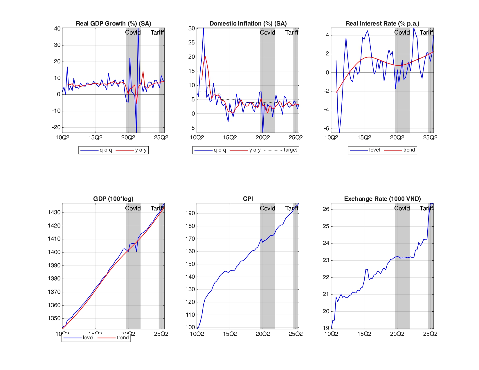
Results from Kalman filtration
The Kalman smoother is applied to the full QPM to jointly estimate all unobserved trends and gaps from Vietnamese data. The figures below show bar decompositions of each endogenous variable into contributions from its structural drivers.
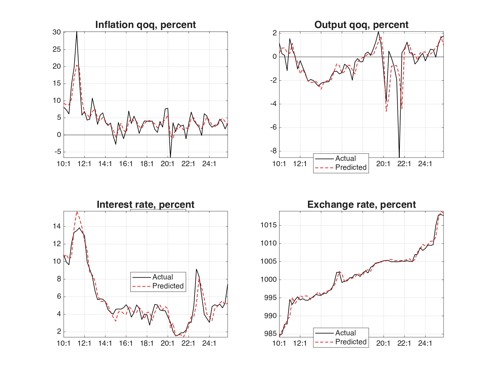
Fitness
Output Gap and MCI Decomposition
The first figure decomposes the output gap (top panel) and the monetary conditions index (bottom panel). The output gap identifies the phases of Vietnam’s business cycle relative to potential.
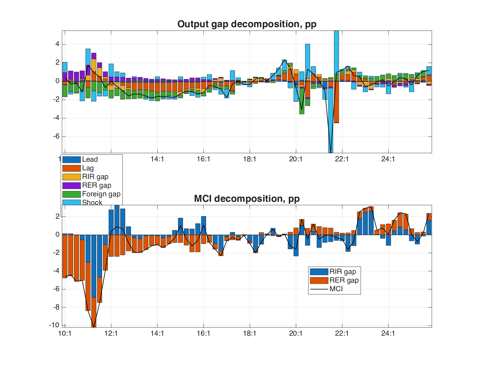
Output gap: The economy ran a mild positive gap through most of 2015–2019, consistent with Vietnam’s strong pre-pandemic growth. The sharpest feature is the large negative output gap around 2021, driven by the Covid-19 shock — the bar decomposition shows this was dominated by the residual shock term rather than policy tightening. Recovery was rapid, with the gap returning close to zero by 2022–2023. The forward-looking (lead) component is small throughout, consistent with the low estimated $b_0$, while the lagged component provides the dominant inertial drag each quarter.
MCI decomposition: The MCI reflects the combined stance of the real interest rate gap (RIR gap) and real exchange rate gap (RER gap). The exchange rate channel (orange bars) dominates throughout the sample, consistent with the low estimated weight of the interest rate in MCI ($b_4 = 0.300$), which assigns a 70% weight to the exchange rate channel. During the Covid period, a real depreciation of the dong eased monetary conditions and partially offset the demand contraction. The interest rate channel (blue bars) became more visible from 2022 onward as the SBV began tightening, but remained the secondary driver.
Marginal Cost and Inflation Decomposition
The second figure decomposes real marginal cost (top panel) and inflation (bottom panel) into structural contributions.
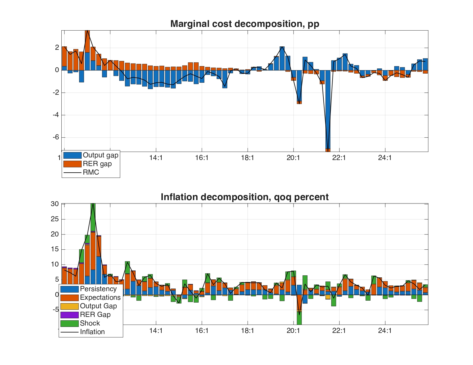
Marginal cost: Real marginal cost is driven primarily by the output gap component, but with a meaningful contribution from the real exchange rate gap (consistent with $a_3 = 0.696$, which assigns approximately 30% weight to imported cost pressures). Cost pressures were negative during 2020–2021 (slack conditions), then turned sharply positive in 2022 as the output gap closed and global commodity prices rose — with both domestic and imported cost channels contributing to the surge.
Inflation decomposition: The post-Covid inflation surge (~2022) is attributed primarily to a large cost-push shock (residual term), rather than to demand overheating or forward inflation expectations alone. Backward-looking persistence (inertia, $a_1 = 0.419$) amplified and prolonged the initial shock. Forward-looking expectations contributed a stabilizing pull toward target once the SBV signaled its inflation-fighting stance. By 2024–2025, all contributions are small and inflation has returned close to the target, consistent with the model’s relatively low inertia estimate.
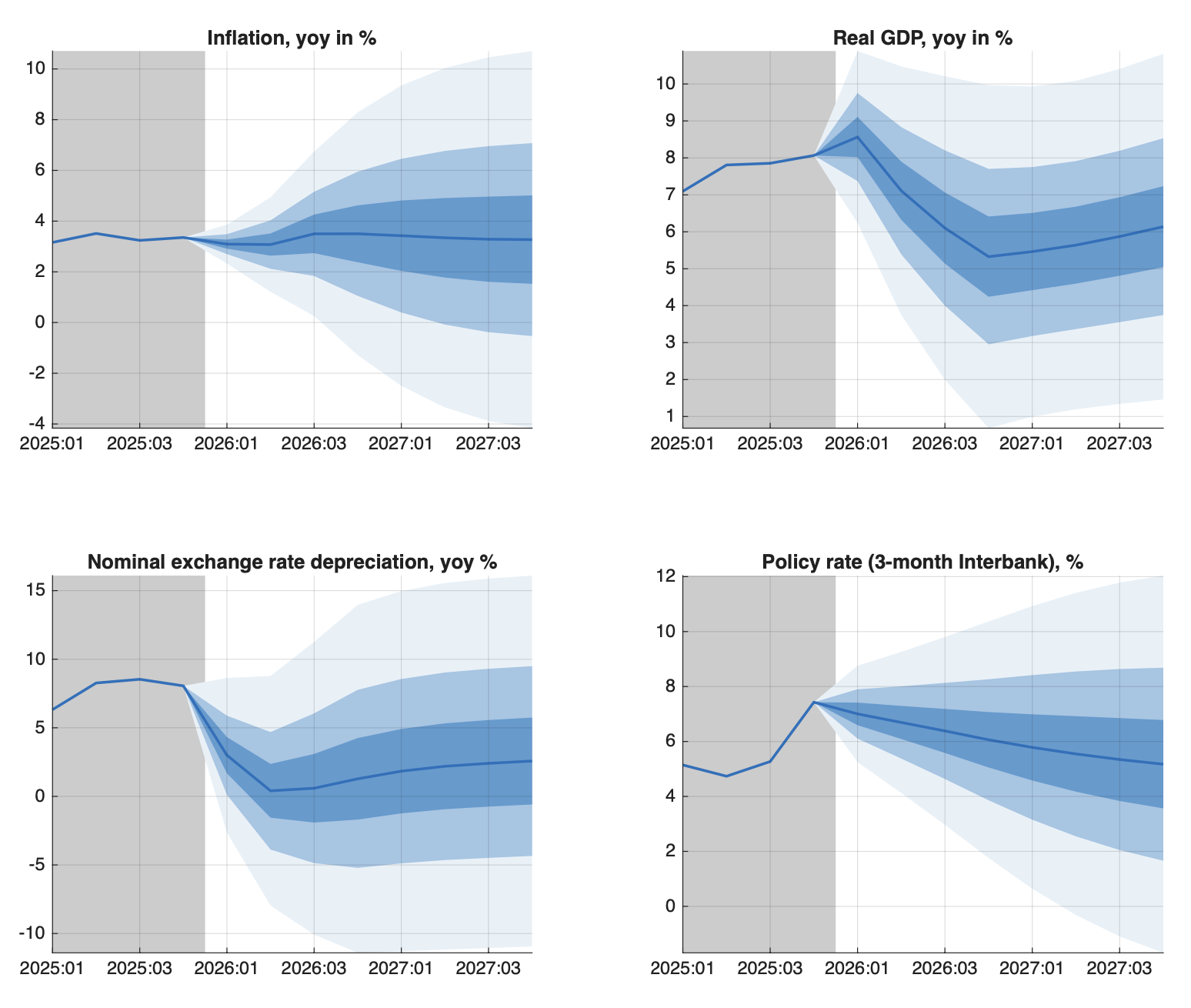
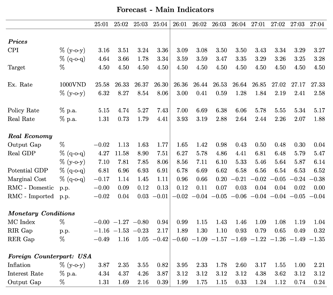
Baseline Forecast
The baseline forecast simulates the model forward from the most recent Kalman-smoothed initial conditions, with foreign-sector variables hard-tuned to assumed external paths (US’ GDP, CPI, Interest rates forecasts are borrowed from Conference Board, dated 2026.03.25). The figures show year-on-year inflation, the output gap, the policy interest rate, and the nominal exchange rate over the forecast horizon. Shaded bands represent fan-chart uncertainty derived from the posterior distribution of shocks.