Notes on RBC calibration
My notes on RBC calibration.
Read more about calibration
- Dynare’s manual
- Computational Methods for Economics
- Chad Fulton’s notes on RBC calibration
- Sims’ note
- Example by Joao Madeira
- ABCs of RBC, King and Rebelo (1999)
Baseline model
Preferences
\[u(C_t,L_t) = \frac{C_t^{1-\sigma}}{1-\sigma} - \frac{L_t^{1+\varphi}}{1+\varphi}\]and a Cobb-Douglas production function
\[Y_t = A_t K_t^\alpha L_t^{1-\alpha}\]The model’s building blocks are
\[C_t^{\sigma} L_t^{\varphi} = W_t, \\ 1 = \beta \mathbb{E}_t\left[ \frac{C_t}{C_{t+1}} (R_{t+1} + 1 - \delta)\right], \\ R_t = \alpha \frac{Y_t}{K_t}, \\ W_t = (1-\alpha)\frac{Y_t}{L_t}, \\ Y_t = A_t K_t^\alpha L_t^{1-\alpha}, \\ K_{t+1} = (1-\delta)K_t + I_t, \\ C_t + I_t = Y_t, \\ A_t = e^{z_t}, z_{t+1} = \rho_A z_t + \varepsilon_t, \varepsilon_t ~ N(0,\sigma^2_A)\]Log-linearized version
\[0 \approx \tilde{Y}_t - \frac{\tilde{L}_t}{1-\overline{L}} - \tilde{C}_t, \\ 0 \approx \tilde{C}_t - \mathbb{E}_t \tilde{C}_{t+1} + \beta \overline{R} \mathbb{E}_t \tilde{R}_{t+1}, \\ 0 \approx \tilde{Y}_t - \tilde{K}_t - \tilde{R}_t, \\ 0 \approx z_t + \alpha \tilde{K}_t + (1-\alpha) \tilde{L}_t - \tilde{Y}_t, \\ 0 \approx \overline{Y}\tilde{Y}_t - \overline{C}\tilde{C}_t + \overline{K}[(1-\delta)\tilde{K}_t - \tilde{K}_{t+1}], \\ z_{t+1} = \rho z_t + \varepsilon_t\]where $\tilde{x}_t = \ln x_t - \ln \overline{x}$.
The steady-state variables $\overline{x}$ can be calculated either by hand or with Dynare.
Dynare codes
The following .mod can be used to solve the model
var Y I C L W R K A;
varexo e;
parameters sigma phi alpha beta delta rhoa;
sigma = 2;
phi = 1.5;
alpha = 0.33;
beta = 0.985;
delta = 0.025;
rhoa = 0.95;
model(linear);
#Rss = (1/beta)-(1-delta);
#Wss = (1-alpha)*((alpha/Rss)^(alpha/(1-alpha)));
#Yss = ((Rss/(Rss-delta*alpha))^(sigma/(sigma+phi))) *(((1-alpha)^(-phi))*((Wss)^(1+phi)))^(1/(sigma+phi));
#Kss = alpha*(Yss/Rss);
#Iss = delta*Kss;
#Css = Yss - Iss;
#Lss = (1-alpha)*(Yss/Wss);
//1-Labor supply
sigma*C + phi*L = W;
//2-Euler equation
(sigma/beta)*(C(+1)-C)=Rss*R(+1);
//3-Law of motion of capital
K = (1-delta)*K(-1)+delta*I;
//4-Production function
Y = A + alpha*K(-1) + (1-alpha)*L;
//5-Demand for capital
R = Y - K(-1);
//6-Demand for labor
W = Y - L;
//7-Equilibrium condition
Yss*Y = Css*C + Iss*I;
//8-Productivity shock
A = rhoa*A(-1) + e;
end;
//-Steady state calculation
steady;
check;
model_diagnostics;
model_info;
//-Shock simulations
shocks;
var e;
stderr 0.01;
end;
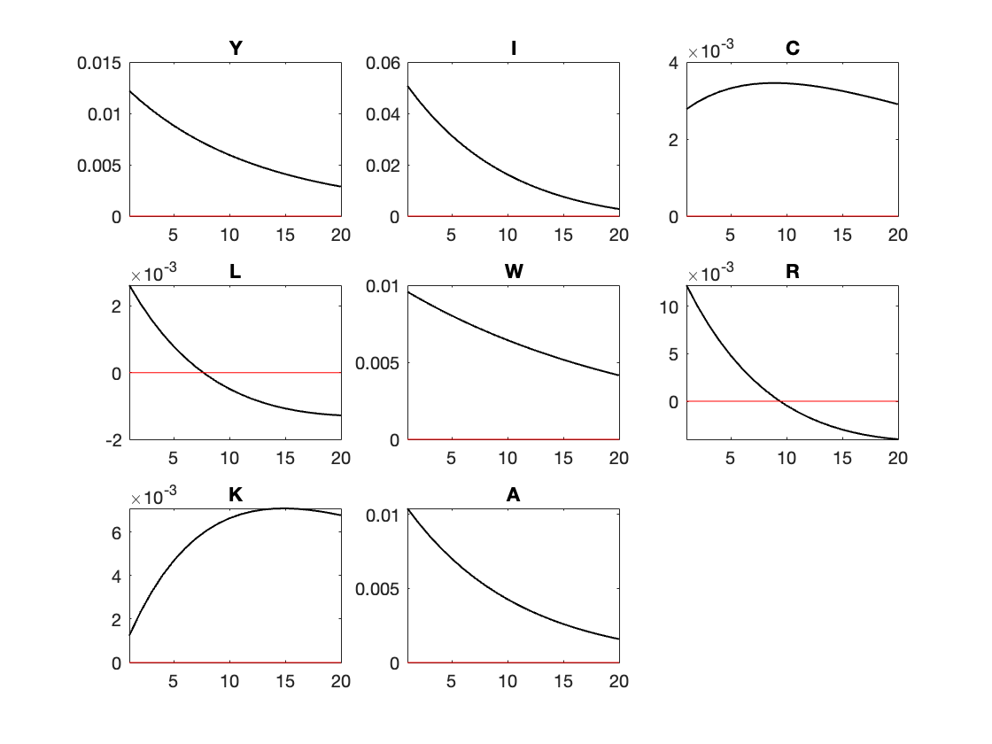
stoch_simul(order=1, irf=20) Y I C L W R K A;
The last line produces the IRF.
To extract the elements for the state-space representation, we can use the following code in MATLAB. (Please read Sims’ note)
% extract the parameters for state-space representation
% variable order: Y I C L W R K A
% state vars: 7, 8
p_Y = 1;
p_I = 2;
p_C = 3;
p_L = 4;
p_W = 5;
p_R = 6;
p_K = 7;
p_A = 8;

% create matrices for the state-space representation
% S(t) = A*S(t-1) + B*e(t)
% X(t) = C*S(t-1) + D*e(t)

A = [   oo_.dr.ghx(oo_.dr.inv_order_var(p_K),:);
        oo_.dr.ghx(oo_.dr.inv_order_var(p_A),:)
    ];
B = [   oo_.dr.ghu(oo_.dr.inv_order_var(p_K),:);
        oo_.dr.ghu(oo_.dr.inv_order_var(p_A),:)
    ];
C = [   oo_.dr.ghx(oo_.dr.inv_order_var(p_Y),:);
        oo_.dr.ghx(oo_.dr.inv_order_var(p_I),:);
        oo_.dr.ghx(oo_.dr.inv_order_var(p_C),:);
        oo_.dr.ghx(oo_.dr.inv_order_var(p_R),:);
        oo_.dr.ghx(oo_.dr.inv_order_var(p_W),:);
        oo_.dr.ghx(oo_.dr.inv_order_var(p_L),:);
    ];
D = [   oo_.dr.ghu(oo_.dr.inv_order_var(p_Y),:);
        oo_.dr.ghu(oo_.dr.inv_order_var(p_I),:);
        oo_.dr.ghu(oo_.dr.inv_order_var(p_C),:);
        oo_.dr.ghu(oo_.dr.inv_order_var(p_R),:);
        oo_.dr.ghu(oo_.dr.inv_order_var(p_W),:);
        oo_.dr.ghu(oo_.dr.inv_order_var(p_L),:);
    ];
Computing IRFs by hand
After the extraction, one can use these values to plot the IRF manually
% compute the impulse reponses by hand
sigma_e = 0.01;
% time horizon
H = 20;
Sirf = zeros(2,H);
Xirf = zeros(6,H);

Sirf(:,1) = B*sigma_e;
Xirf(:,1) = D*sigma_e;

for j = 2:H
    Sirf(:, j) = A*Sirf(:, j-1);
    Xirf(:, j) = C*Sirf(:, j-1);
end

%% Plotting
% Time axis
t = 1:H;

% Variable names for display (including K and A)
% variable order: Y I C L W R K A
var_names = {'Y', 'I', 'C', 'L', 'W', 'R', 'K', 'A'};

% Combine Xirf and Sirf into one matrix for plotting
IRFs_all = [Xirf; Sirf];

% Plot all IRFs
figure;
for i = 1:8
    subplot(3,3,i);
    plot(t, IRFs_all(i,:), 'LineWidth', 1, 'Color','black');
    hold on;
    yline(0, '-k', 'LineWidth', 1, 'Color','r'); % Add horizontal zero line
    hold off;
    title([var_names{i}]);
    %xlabel('Periods');
    %ylabel('Response');
    %grid on;
end

sgtitle('IRFs');
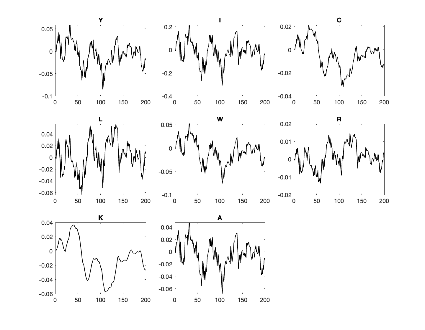
We can also generate the model’s moments based on a random series of shocks.
% compute a simulation. First draw shocks
T = 200;
e = sigma_e * randn(1,T);

Ssim = zeros(2,T);
Xsim = zeros(6,T);

% assume initial state is SS
Ssim(:,1) = B*e(1,1);
for j = 2:T
    Ssim(:,j) = A*Ssim(:,j-1) + B*e(1,j);
    Xsim(:,j) = C*Ssim(:,j-1) + D*e(1,j);
end

% Time axis
t = 1:T;
% Combine Xirf and Sirf into one matrix for plotting
simulated = [Xsim; Ssim];

% Plot all simulated
figure;
for i = 1:8
    subplot(3,3,i);
    plot(t, simulated(i,:), 'LineWidth', 1, 'Color','black');
    title([var_names{i}]);
end
Model Estimation
This exercise is for demonstration only. The data and usage may contain errors.
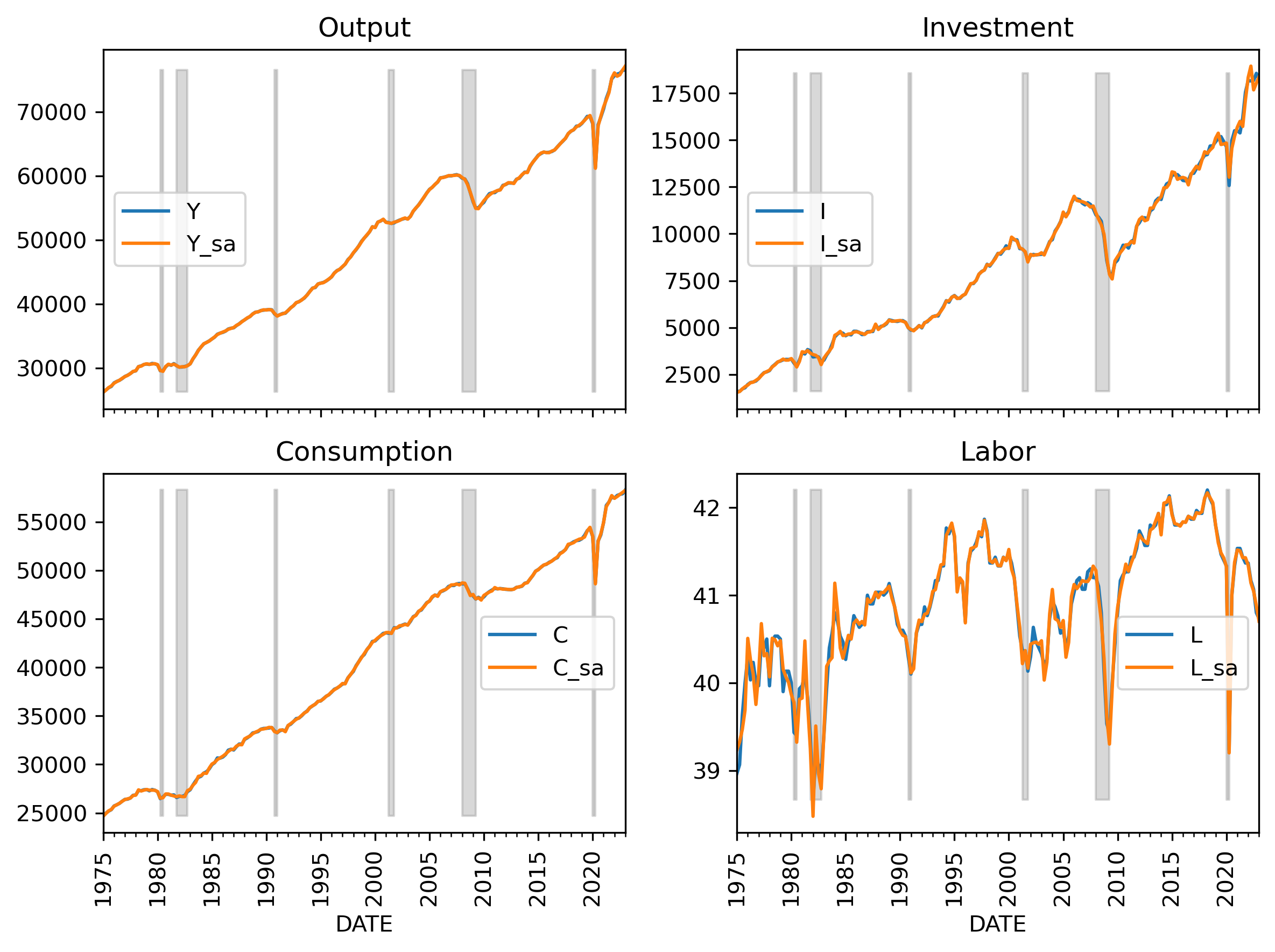
Data retrieval
First, we need some data.
For convenience, let’s use Python. The procedure is:
- Retrieve the data, calculate per-worker for Y,C,I,K,L
- Seasonally adjust all data
- Take logs and calculate the log-difference
- Then demean these values (so that we have a data matched with the model’s steady state)
# library
from pandas_datareader.data import DataReader
import pandas as pd
import numpy as np
import matplotlib.pyplot as plt
from statsmodels.tsa.seasonal import STL
from statsmodels.tsa.filters.hp_filter import hpfilter

# Get some data
start='1975-01'
end = '2023-03'

labor = DataReader('HOHWMN02USQ065S', 'fred', start=start, end=end)         # hours
consumption = DataReader('PCECC96', 'fred', start=start, end=end)           # billions of dollars
investment = DataReader('GPDI', 'fred', start=start, end=end)               # billions of dollars
capital = DataReader('NFIRSAXDCUSQ', 'fred', start=start, end=end)          # million of dollars
population = DataReader('CNP16OV', 'fred', start=start, end=end)            # thousands of persons
# shading for recession
recessions = DataReader('USRECQ', 'fred', start=start, end=end)
recessions = recessions.resample('QS').last()['USRECQ'].iloc[1:]

# Collect the raw values
raw = pd.concat((labor, consumption, investment, capital, population.resample('QS').mean()), axis=1)
raw.columns = ['labor', 'consumption', 'investment','capital', 'population']
raw['output'] = raw['consumption'] + raw['investment']

# convert data to units and normalize with population
y = (raw['output'] * 1e9) / (raw['population'] * 1e3)
i = (raw['investment'] * 1e9) / (raw['population'] * 1e3)
c = (raw['consumption'] * 1e9) / (raw['population'] * 1e3)
k = (raw['capital'] * 1e12)/(raw['population']*1e3)
h = raw['labor']

# assemble into 1 dataset
dta = pd.DataFrame({
    'Y': y,
    'I': i,
    'C': c,
    'L': h,
    'K': k
})
# transform date to a new column with YYYYQQ format
dta['dynare_date'] = dta.index.to_period('Q').astype(str).str.replace('-', 'Q')
dta['recession'] = recessions

# Apply the STL decomposition on Y, I, C, L, K
def stl_decompose(series):
    raw = series.dropna()
    stl = STL(raw, period=4, robust=True)
    res = stl.fit()
    adjusted = raw - res.seasonal
    return adjusted

# Extract the seasonally adjusted data
dta['Y_sa'] = stl_decompose(dta['Y'])
dta['I_sa'] = stl_decompose(dta['I'])
dta['C_sa'] = stl_decompose(dta['C'])
dta['L_sa'] = stl_decompose(dta['L'])
dta['K_sa'] = stl_decompose(dta['K'])

# take logs
dta['logY_sa'] = np.log(dta['Y_sa'])
dta['logI_sa'] = np.log(dta['I_sa'])
dta['logC_sa'] = np.log(dta['C_sa'])
dta['logL_sa'] = np.log(dta['L_sa'])
dta['logK_sa'] = np.log(dta['K_sa'])
# calculate the differences in logY_sa, logI_sa, logC_sa, logL_sa, logK_sa
dta['dY_sa'] = dta['logY_sa'].diff()
dta['dI_sa'] = dta['logI_sa'].diff()
dta['dC_sa'] = dta['logC_sa'].diff()
dta['dL_sa'] = dta['logL_sa'].diff()
# demean the log values
dta['dy'] = dta['dY_sa'] - dta['dY_sa'].mean()
dta['di'] = dta['dI_sa'] - dta['dI_sa'].mean()
dta['dc'] = dta['dC_sa'] - dta['dC_sa'].mean()
dta['dl'] = dta['dL_sa'] - dta['dL_sa'].mean()
# apply the Hodrick-Prescott filter to the log values
from statsmodels.tsa.filters.hp_filter import hpfilter
dta['Y_hp_cyc'], dta['Y_hp_trend'] = hpfilter(dta['logY_sa'], lamb=1600)
dta['I_hp_cyc'], dta['I_hp_tred'] = hpfilter(dta['logI_sa'], lamb=1600)
dta['C_hp_cyc'], dta['C_hp_tred'] = hpfilter(dta['logC_sa'], lamb=1600)
dta['L_hp_cyc'], dta['L_hp_tred'] = hpfilter(dta['logL_sa'], lamb=1600)
dta['K_hp_cyc'], dta['K_hp_tred'] = hpfilter(dta['logK_sa'], lamb=1600)
# calculate differences of the HP filtered values
dta['dy_hp'] = dta['Y_hp_cyc'].diff()
dta['di_hp'] = dta['I_hp_cyc'].diff()
dta['dc_hp'] = dta['C_hp_cyc'].diff()
dta['dl_hp'] = dta['L_hp_cyc'].diff()
# make sure dta'DATES is the first column
dta = dta.reset_index()
dta = dta[['DATES', 'Y', 'I', 'C', 'L', 'K', 'Y_sa', 'I_sa', 'C_sa', 'L_sa', 'K_sa',
           'logY_sa', 'logI_sa', 'logC_sa', 'logL_sa', 'logK_sa',
           'dY_sa', 'dI_sa', 'dC_sa', 'dL_sa',
           'dy', 'di', 'dc', 'dl',
           'Y_hp_cyc', 'Y_hp_trend',
           'I_hp_cyc', 'I_hp_tred',
           'C_hp_cyc', 'C_hp_tred',
           'L_hp_cyc', 'L_hp_tred',
           'K_hp_cyc', 'K_hp_tred',
           'dy_hp', 'di_hp', 'dc_hp', 'dl_hp',
           'recession']]
# Save the data to an excel file
# save data
dta.to_csv(usdat.csv, index=False)
Estimation
This procedure can be done in Dynare by adding two things to the .mod file.
- a measurement variable
dy(we take changes in log output as the observed data) - add one more identity equation to the
modelblock - estimate the model’s parameters using Bayesian methods
- decompose the shock from data and save it to an
xlsfile. (for estimation, burn the first 8 obs)
// ------ variable list
var Y I C L W R K A dy;

model(linear);
.
.
.
//9-measurement identity
dy = Y-Y(-1);
end;

// ---------- Observed variables ----------
varobs dy;

// ---------- Priors for Bayesian estimation ----------
estimated_params;
sigma,      2,	                NORMAL_PDF, 2, 0.05;
phi,        1.5,                NORMAL_PDF, 1.5, 0.1;
alpha,      0.33,               NORMAL_PDF, 0.3, 0.05;
beta,       0.99,               beta_pdf, 0.985, 0.005;
rhoa,       0.95,               beta_pdf, 0.95, 0.02;
stderr e,   0.02,               inv_gamma_pdf, 0.01, 2;
end;

// ---------- Estimation command ----------
estimation(
  datafile=usdat,
  first_obs=8,
  presample=4,
  lik_init=2,
  mode_check,
  prefilter=0,
  mh_replic=250000,
  mh_nblocks=2,
  mh_jscale=1.08,
  mh_drop=0.2
);

// ---------- Shock decomposition ----------
shock_decomposition(datafile=usdat, first_obs=8) dy;
plot_shock_decomposition(write_xls) dy;
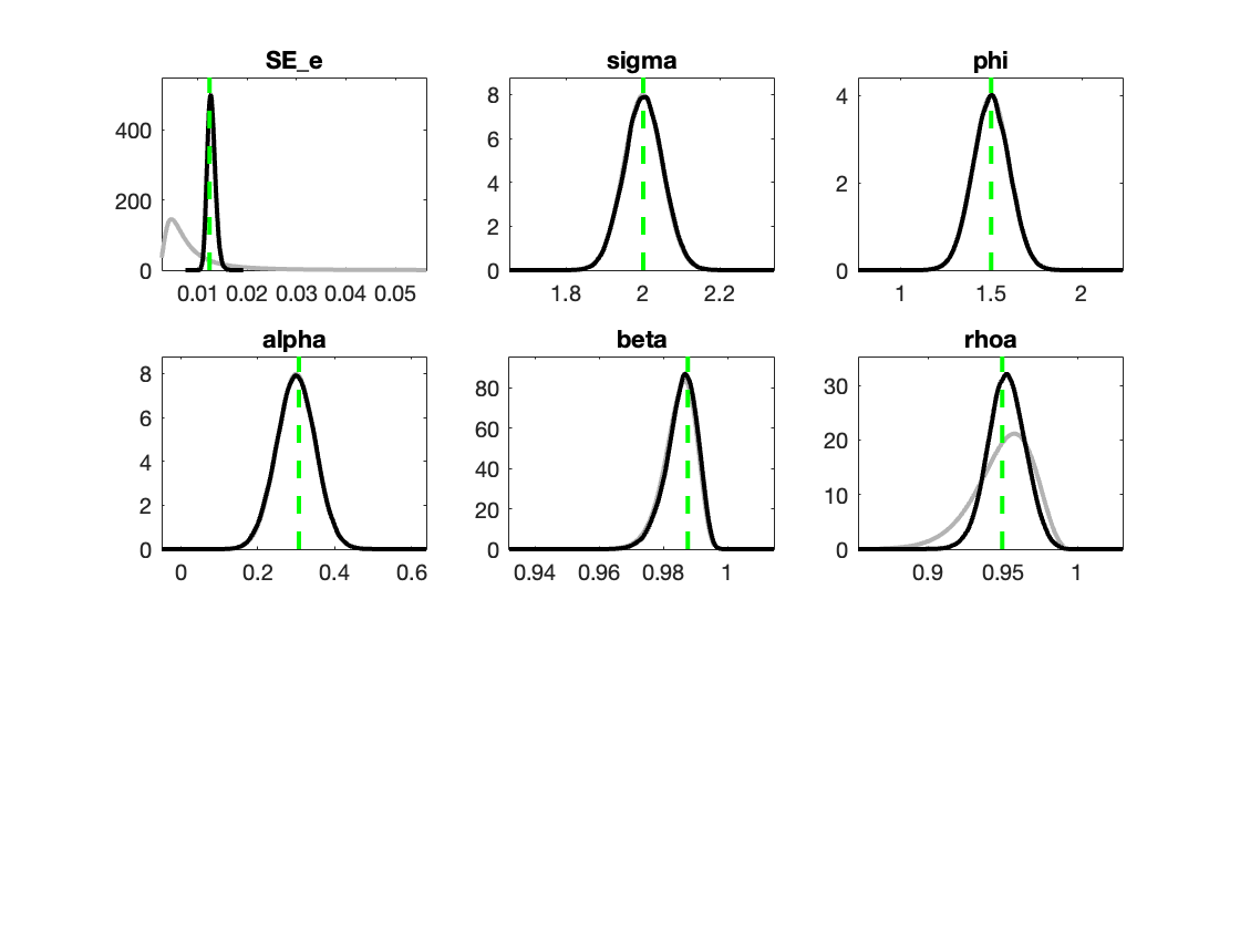
| Parameter | Prior Mean | Posterior Mean | 90% HPD Interval | Prior | Std. Dev. |
|---|---|---|---|---|---|
| sigma | 2.000 | 2.0008 | [1.2735, 2.8675] | norm | 0.5000 |
| phi | 1.500 | 1.4982 | [0.9421, 1.9585] | norm | 0.3000 |
| alpha | 0.330 | 0.2986 | [0.2291, 0.3925] | beta | 0.0500 |
| beta | 0.985 | 0.9854 | [0.9775, 0.9932] | beta | 0.0050 |
| rhoa | 0.950 | 0.9523 | [0.8591, 0.9498] | beta | 0.0200 |
| e | 0.010 | 0.0127 | [0.0114, 0.0140] | invg | 2.0000 |
We can re-run the model with the Bayesian updated parameters.
Eyeball Simulation
Aside from statistical checks, one can also simulate the model based on a given series of shocks.
Using the data from decomposition, we can produce an image like this.
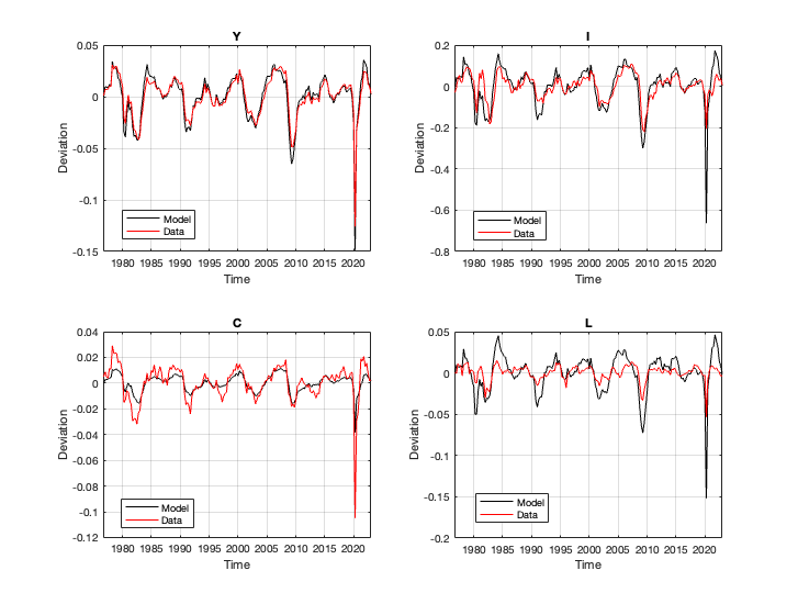
The replication codes are stored here.